
by Svetlana Cheusheva , updated on March 21, 2023
The tutorial shows 3 different techniques to plot a histogram in Excel - using the special Histogram tool of Analysis ToolPak, FREQUENCY or COUNTIFS function, and PivotChart.
While everyone knows how easy it is to create a chart in Excel, making a histogram usually raises a bunch of questions. In fact, in the recent versions of Excel, creating a histogram is a matter of minutes and can be done in a variety of ways - by using the special Histogram tool of the Analysis ToolPak, formulas or the old good PivotTable. Further on in this tutorial, you will find the detailed explanation of each method.
Wikipedia defines a histogram in the following way: "Histogram is a graphical representation of the distribution of numerical data." Absolutely true, and… totally unclear :) Well, let's think about histograms in another way.
Have you ever made a bar or column chart to represent some numerical data? I bet everyone has. A histogram is a specific use of a column chart where each column represents the frequency of elements in a certain range. In other words, a histogram graphically displays the number of elements within the consecutive non-overlapping intervals, or bins.
For example, you can make a histogram to display the number of days with a temperature between 61-65, 66-70, 71-75, etc. degrees, the number of sales with amounts between $100-$199, $200-$299, $300-$399, the number of students with test scores between 41-60, 61-80, 81-100, and so on.
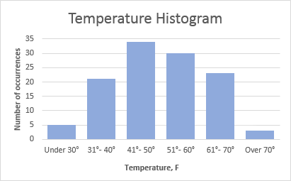
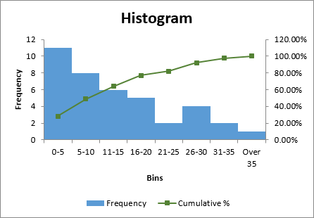
The following screenshot gives an idea of how an Excel histogram can look like:
The Analysis ToolPak is a Microsoft Excel data analysis add-in, available in all modern versions of Excel beginning with Excel 2007. However, this add-in is not loaded automatically on Excel start, so you would need to load it first.
To add the Data Analysis add-in to your Excel, perform the following steps:
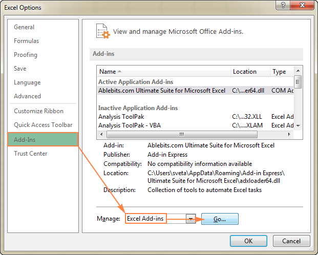

Now, the Analysis ToolPak is loaded in your Excel, and its command is available in the Analysis group on the Data tab.
Before creating a histogram chart, there is one more preparation to make - add the bins in a separate column.
Bins are numbers that represent the intervals into which you want to group the source data (input data). The intervals must be consecutive, non-overlapping and usually equal size.
Excel's Histogram tool includes the input data values in bins based on the following logic:
Considering the above, type the bin numbers that you want to use in a separate column. The bins must be entered in ascending order, and your Excel histogram bin range should be limited to the input data range.
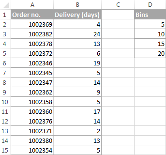
In this example, we have order numbers in column A and estimated delivery in column B. In our Excel histogram, we want to display the number of items delivered in 1-5 days, 6-10 days, 11-15 days, 16-20 days and over 20 days. So, in column D, we enter the bin range from 5 to 20 with an increment of 5 as shown in the below screenshot:
With the Analysis ToolPak enabled and bins specified, perform the following steps to create a histogram in your Excel sheet:


Tip. If you included column headers when selecting the input data and bin range, select the Labels check box.
For this example, I've configured the following options: 

Tip. To improve the histogram, you can replace the default Bins and Frequency with more meaningful axis titles, customize the chart legend, etc. Also, you can use the design, layout, and format options of the Chart Tools to change the display of the histogram, for example remove gaps between columns. For more details, please see How to customize and improve Excel histogram.
As you've just seen, it's very easy to make a histogram in Excel using the Analysis ToolPak. However, this method has a significant limitation - the embedded histogram chart is static, meaning that you will need to create a new histogram every time the input data is changed.
To make an automatically updatable histogram, you can either use Excel functions or build a PivotTable as demonstrated below.
Another way to create a histogram in Excel is using the FREQUENCY or COUNTIFS function. The biggest advantage of this approach is that you won't have to re-do your histogram with each change in the input data. Like a normal Excel chart, your histogram will update automatically as soon as you edit, add new or delete existing input values.

To begin with, arrange your source data in one column (column B in this example), and enter the bin numbers in another column (column D), like in the screenshot below:
Now, we will use a Frequency or Countifs formula to calculate how many values fall into the specified ranges (bins), and then, we will draw a histogram based on that summary data.
The most obvious function to create a histogram in Excel is the FREQUENCY function that returns the number of values that fall within specific ranges, ignoring text values and blank cells.
The FREQUENCY function has the following syntax:
FREQUENCY(data_array, bins_array)In this example, the data_array is B2:B40, bin array is D2:D8, so we get the following formula:
Please keep in mind that FREQUENCY is a very specific function, so follow these rules to make it work right:
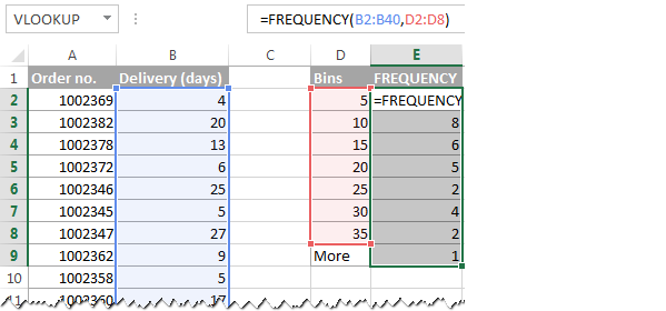
Like the Histogram option of the Analysis ToolPak, the Excel FREQUENCY function returns values that are greater than a previous bin and less than or equal to a given bin. The last Frequency formula (in cell E9) returns the number of values greater than the highest bin (i.e. the number of delivery days over 35).

To make things easier to understand, the following screenshot shows the bins (column D), corresponding intervals (column C), and computed frequencies (column E):
Note. Because Excel FREQUENCY is an array function, you cannot edit, move, add or delete the individual cells containing the formula. If you decide to change the number of bins, you will have to delete the existing formula first, then add or delete the bins, select a new range of cells, and re-enter the formula.
Another function that can help you calculate frequency distributions to plot histogram in Excel is COUNTIFS. And in this case, you will need to use 3 different formulas:
Tip. If you plan to add more input data rows in the future, you can supply a bigger range in your FREQUENCY or COUNTIFS formulas, and you won't have to change your formulas as you add more rows. In this example, the source data are in cells B2:B40. But you can supply the range B2:B100 or even B2:B1000, just in case :) For example: =FREQUENCY(B2:B1000,D2:D8)
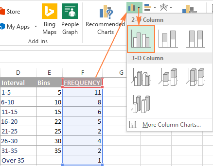
Now that you have a list of frequency distributions computed with either FREQUENCY or COUNTIFS function, create a usual bar chart - select the frequencies, switch to the Insert tab and click the 2-D Column chart in the Charts group:
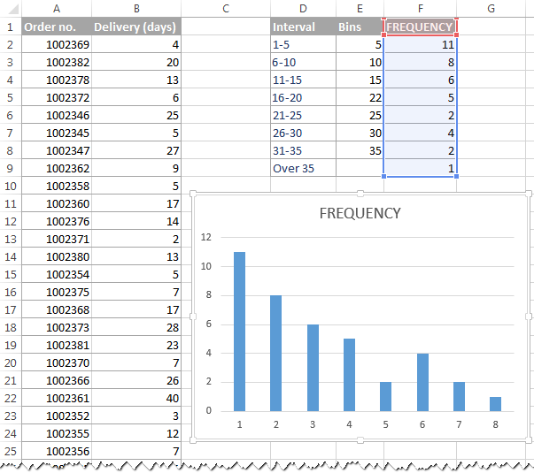
 The bar graph will be immediately inserted in your sheet:
 Generally speaking, you already have a histogram for your input data, though it definitely requires a few improvements. Most importantly, to make your Excel histogram easy to understand, you need to replace the default labels of the horizontal axis represented by serial numbers with your bin numbers or ranges. The easiest way is to type the ranges in a column left to the column with the Frequency formula, select both columns - Ranges and Frequencies - and then create a bar chart. The ranges will be automatically used for the X axis labels, as shown in the below screenshot:
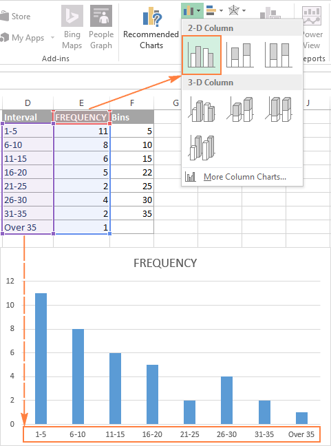
Tip. If Excel converts your intervals to dates (e.g. 1-5 can be automatically converted to 05-Jan), then type the intervals with a preceding apostrophe (') like '1-5. If you want the labels of your Excel histogram to display bin numbers, type them with preceding apostrophes too, e.g. '5, '10, etc. The apostrophe just converts numbers to text and is invisible in cells and on the histogram chart.
If there is no way you can type the desired histogram labels on your sheet, then you can enter them directly on the chart, independently of the worksheet data. The final part of this tutorial explains how to do this, and shows a couple of other improvements that can be made to your Excel histogram.

As you may have noticed in the two previous examples, the most time-consuming part of creating a histogram in Excel is calculating the number of items within each bin. Once the source data has been grouped, an Excel histogram chart is fairly easy to draw. As you probably know, one of the fastest ways to automatically summarize data in Excel is a PivotTable. So, let's get to it and plot a histogram for the Delivery data (column B):

To create a pivot table, go to the Insert tab > Tables group, and click PivotTable. And then, move the Delivery field to the ROWS area, and the other field (Order no. in this example) to the VALUES area, as shown in the below screenshot. If you have not dealt with Excel pivot tables yet, you may find this tutorial helpful: Excel PivotTable tutorial for beginners.
By default, numeric fields in a PivotTable are summed, and so is our Order numbers column, which makes absolutely no sense :) Anyway, because for a histogram we need a count rather than sum, right-click any order number cell, and select Summarize Values By > Count.
 Now, your updated PivotTable should look like this:
The next step is to create the intervals, or bins. For this, we will be using the Grouping option. Right-click any cell under Row Labels in your pivot table, and select Group… In the Grouping dialog box, specify the starting and ending values (usually Excel enters the minimum and maximum value automatically based on your data), and type the desired increment (interval length) in the By box. In this example, the minimum delivery time is 1 day, maximum - 40 days, and the increment is set to 5 days:
 Click OK, and your pivot table will display the intervals as specified:
One final step is left - draw a histogram. To do this, simply create a column pivot chart by clicking the PivotChart on the Analyze tab in PivotTable Tools group:  And the default column PivotChart will appear in your sheet straight away:
  And now, polish up your histogram with a couple of finishing touches:

Additionally, you may want to achieve a conventional histogram look where bars touch each other. And you will find the detailed guidance on how to do this in the next and final part of this tutorial.
Whether you create a histogram using the Analysis ToolPak, Excel functions or a PivotChart, you might often want to customize the default chart to your liking. We have a special tutorial about Excel charts that explains how to modify the chart title, legend, axes titles, change the chart colors, layout and style. And here, we will discuss a couple of major customizations specific to an Excel histogram.
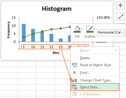
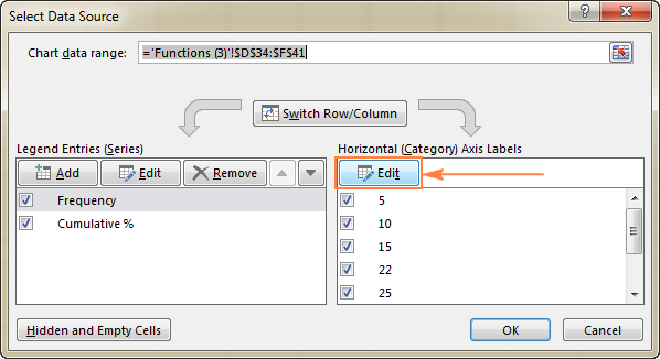
When creating a histogram in Excel with the Analysis ToolPak, Excel adds the horizontal axis labels based on the bin numbers that you specify. But what if, on your Excel histogram graph, you want to display ranges instead of bin numbers? For this, you'd need to change the horizontal axis labels by performing these steps:


When making a histogram in Excel, people often expect adjacent columns to touch each other, without any gaps. This is an easy thing to fix. To eliminate empty space between the bars, just follow these steps:


And voila, you have plotted an Excel histogram with bars touching each other:
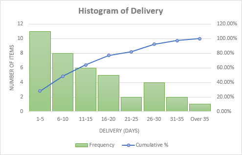
And then, you can embellish your Excel histogram further by modifying the chart title, axes titles, and changing the chart style or colors. For example, your final histogram may look something like this:
This is how you draw a histogram in Excel. For better understanding of the examples discussed in this tutorial, you can download the sample Excel Histogram sheet with source data and histogram charts. I thank you for reading and hope to see you on our blog next week.